‘모델 훈련’을 위한 준비
배경지식
편미분, 벡터, 행렬, 회귀분석 내용을 아는 것이 필요하다.
np.random.rand : [0, 1] 인 균일분포에서 난수 행렬 생성
np.random.randn : 표준정규분포에서 난수 행렬 생성
코드
먼저 몇 개의 모듈을 import 해야 한다.
import numpy as np
import pandas as pd
import matplotlib.pyplot as plt
import matplotlib as mpl
import sklearn
import os


np.random.seed(42)
mpl.rc('axes', labelsize = 14)
mpl.rc('xtick', labelsize = 12)
mpl.rc('ytick', labelsize = 12)
1. 선형회귀
1. 정규방정식
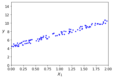
X = 2 * np.random.rand(100, 1)
y = 4 + 3 * X + np.random.rand(100, 1)
plt.plot(X, y, "b.")
plt.xlabel("$X_1$")
plt.ylabel("$y$", rotation=0)
plt.axis([0, 2, 0, 15])
plt.show()
\hat\theta = (X^TX)^{-1}X^Ty
X_b = np.c_[np.ones((100, 1)), X]
theta_best = np.linalg.inv(X_b.T.dot(X_b)).dot(X_b.T).dot(y)
theta_best

>>> array([[4.51359766],
		       [2.98323418]])
y = 4 + 3x + 가우시안 잡음 이라는 함수를 사용.
\theta_{0} = 4\text{와}\; \theta_{1} = 3를 기대함.
그러나 현실은 그렇지 못함. (잡음 때문에)
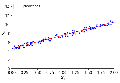
\hat\theta를 사용해 예측 \hat y = X\hat\theta
X_new = np.array([[0], [2]])
X_new_b = np.c_[np.ones((2, 1)), X_new]
y_predict = X_new_b.dot(theta_best)
y_predict
plt.plot(X_new, y_predict, "r-", label="predictions")
plt.plot(X, y, "b.")
plt.axis([0, 2, 0, 15])
plt.xlabel("$X_1$")
plt.ylabel("$y$", rotation=0)
plt.legend(loc='upper left')
plt.show()
2. 사이킷런으로 선형 회귀 해보기
from sklearn.linear_model import LinearRegression
lin_reg = LinearRegression()
lin_reg.fit(X, y)
lin_reg.intercept_, lin_reg.coef_

>>> (array([4.51359766]), array([[2.98323418]]))
- LinearRegression 클래스는 scipy.linalg.lstsq()함수에서 따온 것. (lstsq = 최소제곱) \
- 이 함수는 \hat\theta = X^{+}y를 직접 계산한다.
X^{+}는 X의 유사역행렬(무어-팬로즈 역행렬).
theta_best_svd, residuals, rank, s = np.linalg.lstsq(X_b, y, rcond=1e-6)
theta_best_svd

>>> array([[4.51359766],
		       [2.98323418]])
- np.linalg.pinv() 함수로 유사역행렬 계산 가능하다.
np.linalg.pinv(X_b).dot(y)

>>> array([[4.51359766],
		       [2.98323418]])
3. 선형회귀와 계산 복잡도
- 선형 회귀는 간단하고, 예측이 빠르다.
- 그러나 샘플수와 특성수에 계산 복잡도가 선형적인 단점을 가지고 있다.
- 즉, 샘플이 늘어나면 계산 속도도 느려진다.
2. 경사하강법
비용함수를 최소화하기 위해 파라미터를 반복적으로 조정하는 기법
\theta를 임의의 값에서 시작해서 조금씩 비용함수 값이 감소되는 방향으로 이동하는 것.
스텝의 크기가 가장 중요한 파라미터. 학습률 하이퍼파라미터로 결정된다.
학습률이 너무 작으면 너무 반복이 시간이 많이 걸린다.
학습률이 너무 높으면 골짜기를 가로질러 비용함수 값이 오히려 발산할 수도 있다.
1. 배치 경사 하강법
매번 스텝을 밟을 때마다 전체 훈련 세트에 대해 계산. 매우 큰 훈련세트에서는 굉장히 느리다.
단, 특성 수에는 민감하지 않다.
\eta : 에타라고 읽는다.
2. 확률적 경사 하강법(SGD)
매 스텝에서 한 개의 샘플을 무작위로 선택하고, 그 하나의 샘플에 대한 그레이디언트를 계산.
알고리즘이 좀 더 빠르게 작동할 수 있음.
또한 하나의 샘플만 있으면 되므로 큰 훈련세트도 훈련시킬 수 있음.
단, 무작위로 작동하므로 배치 경사하강법보다 훨씬 더 불안정하다는 단점이 있음.
- 비용함수가 위 아래로 요동치며
3. 미니 배치 모델
theta_path_mgd = []

n_iterations = 50
minibatch_size = 20

np.random.seed(42)
theta = np.random.randn(2,1)  # 랜덤 초기화

t0, t1 = 200, 1000
def learning_schedule(t):
    return t0 / (t + t1)

t = 0
for epoch in range(n_iterations):
    shuffled_indices = np.random.permutation(m)
    X_b_shuffled = X_b[shuffled_indices]
    y_shuffled = y[shuffled_indices]
    for i in range(0, m, minibatch_size):
        t += 1
        xi = X_b_shuffled[i:i+minibatch_size]
        yi = y_shuffled[i:i+minibatch_size]
        gradients = 2/minibatch_size * xi.T.dot(xi.dot(theta) - yi)
        eta = learning_schedule(t)
        theta = theta - eta * gradients
        theta_path_mgd.append(theta)
theta

>>> array([[4.52651397],
		       [2.99723869]])
theta_path_bgd = np.array(theta_path_bgd)
theta_path_sgd = np.array(theta_path_sgd)
theta_path_mgd = np.array(theta_path_mgd)

plt.figure(figsize=(7,4))
plt.plot(theta_path_sgd[:, 0], theta_path_sgd[:, 1], "r-s", linewidth=1, label="Stochastic")
plt.plot(theta_path_mgd[:, 0], theta_path_mgd[:, 1], "g-+", linewidth=2, label="Mini-batch")
plt.plot(theta_path_bgd[:, 0], theta_path_bgd[:, 1], "b-o", linewidth=3, label="Batch")
plt.legend(loc="upper left", fontsize=16)
plt.xlabel(r"$\theta_0$", fontsize=20)
plt.ylabel(r"$\theta_1$   ", fontsize=20, rotation=0)
plt.axis([2.5, 4.5, 2.3, 3.9])
plt.show()
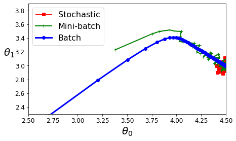
선형회귀를 사용한 알고리즘의 비교
3. 다항회귀
- 단순한 직선보다 복잡한 형태일 경우 사용한다.
- 각 특성의 거듭제곱을 새로운 특성으로 추가하고, 확장된 특성을 포함하는
데이터셋에 선형 모델을 훈련시키면 됨.
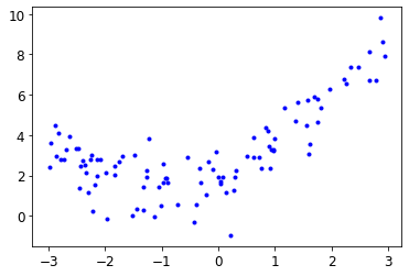
- 2차방정식으로 비선형 데이터 생성
m = 100
X = 6 * np.random.rand(m, 1) - 3
y = 0.5 * X**2 + X + 2 + np.random.randn(m, 1)
plt.plot(X, y, "b.")
X = matrix
(\text{잔차}) = matrix
y = 0.5X^{2} + X + 2 + (\text{잔차})
-
non-linear model 만들기
pythonfrom sklearn.preprocessing import PolynomialFeatures poly_features = PolynomialFeatures(degree = 2, include_bias = False) X_poly = poly_features.fit_transform(X) X[0] >>> array([-1.4436696]) X_poly[0] >>> array([-1.4436696, 2.0841819])linear regression 적용해보기
pythonlin_reg.fit(X_poly, y) lin_reg.intercept_, lin_reg.coef_ >>> (array([1.96301211]), array([[0.94048827, 0.48463253]])) -
그래프 만들기
pythonX_new = np.linspace(-3, 3, 100).reshape(100, 1) X_new_poly = poly_features.transform(X_new) y_new = lin_reg.predict(X_new_poly) plt.plot(X, y, "b.") plt.plot(X_new, y_new, "r-", linewidth=2, label="Predictions") plt.xlabel("$x_1$", fontsize=18) plt.ylabel("$y$", rotation=0, fontsize=18) plt.legend(loc="upper left", fontsize=14) plt.axis([-3, 3, 0, 10]) plt.show()
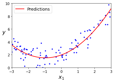
- 실제 vs 예측
- 실제 식:
- 예측 식:
- 특성이 여러 개인 경우, 다항 회귀는 이 특성 사이의 관계를 찾을 수 있음.
4. 학습 곡선
1. n차 다항회귀
- 고차 다항회귀를 적용하면 보통 선형회귀보다 더 데이터에 적합하게 맞출 수 있음.
- 그러나, 이는 심각하게 과대적합된 것이라고 평가할 수도 있음.
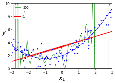
1차 vs 2차 vs 300차
- 1차 모델: 과소적합
- 2차 모델: 가장 일반화가 잘됨.
- 300차 모델: 과대적합
해당 그래프의 코드
from sklearn.preprocessing import StandardScaler
from sklearn.pipeline import Pipeline

for style, width, degree in (("g-", 1, 300), ("b--", 2, 2), ("r-+", 2, 1)):
    polybig_features = PolynomialFeatures(degree=degree, include_bias=False)
    std_scaler = StandardScaler()
    lin_reg = LinearRegression()
    polynomial_regression = Pipeline([
            ("poly_features", polybig_features),
            ("std_scaler", std_scaler),
            ("lin_reg", lin_reg),
        ])
    polynomial_regression.fit(X, y)
    y_newbig = polynomial_regression.predict(X_new)
    plt.plot(X_new, y_newbig, style, label=str(degree), linewidth=width)

plt.plot(X, y, "b.", linewidth=3)
plt.legend(loc="upper left")
plt.xlabel("$x_1$", fontsize=18)
plt.ylabel("$y$", rotation=0, fontsize=18)
plt.axis([-3, 3, 0, 10])
plt.show()
2. 과대적합 극복하기: 학습곡선
- ㄴㅁㅇㄹㅁㄴㅇㄹ
- ㅁㄴㅇㄹㄴㅁㅇㄹㅁㄴㅇ
from sklearn.metrics import mean_squared_error
from sklearn.model_selection import train_test_split

def plot_learning_curves(model, X, y):
  X_train, X_val, y_train, y_val = train_test_split(X, y, test_size = 0.2)
  train_errors, val_errors = [], []
  for m in range(1, len(X_train)):
    model.fit(X_train[:m], y_train[:m])
    y_train_predict = model.predict(X_train[:m])
    y_val_predict = model.predict(X_val)
  plt.plot(np.sqrt(train_errors), "r-+", linewidth = 2, label="훈련 세트")
  plt.plot(np.sqrt(val_errors), "b-", linewidth=3, label="검증 세트")
lin_reg = LinearRegression()
plot_learning_curves(lin_reg, X, y)
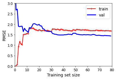
과소 적합 모델 그리기