주요 단계
- 큰 그림
- 데이터 구하기
- 탐색, 시각화
- 데이터 준비
- 모델 선택 & 훈련
- 솔루션 제시
- 시스템 론칭, 모니터링, 유지보수
1. 데이터로 작업하기
다양한 공개 데이터 저장소
http://archive.ics.uci.edu/ml
http://www.kaggle.com/datasets
https://registry.opendata.aws

http://dataportals.org
http://opendatamonitor.eu
http://quandl.com

https://goo.gl/SJHN2k
https://homl.info/10
http://www.reddit.com/r/datasets

https://goo.gl/QgRbUL
2. 큰 그림 보기
문제 정의
어떠한 문제를 해결할 것인가?
성능 측정 지표 선택
크게 2가지 예시를 들고 있다.
- RMSE = root mean square error = 평균 제곱근 오차
- X= 행렬
- h = 예측 함수
- \underline{x}^{(i)} = 행렬 X의 i번째 행.
- y^{(i)} = 기댓값
- h(\underline{x}^{(i)}) = \hat y = 추정량임.
- \hat y - y 를 제곱한 것 <=> 잔차제곱의 합
즉, RMSE 는 잔차제곱의 합을 샘플 수로 나눈 것에 제곱근을 씌운 것.
-
MAE = mean absolute error
MAE(X, h) = \frac {1}{m} \sum_{i=1}^{m} |h(\underline{x}^{(i)})-y^{(i)}|
두 방향 모두 예측값 벡터와 타깃값 벡터의 거리를 제는 방법 (=잔차제곱합)
가정 검사
지금까지의 가정이 맞는가 확인
3. 데이터 가져오기
1. 파이썬 설치 :
- 스파이더 설정하기
- 구글 코랩도 괜찮다.
- 주피터 노트북 설정하기
Untitled
2. 데이터 끌어들이기
- 여기서는 캘리포니아의 주택 가격 데이터를 사용한다.
코드
데이터 잡아오기 (fetch)
import os
import tarfile
import urllib.request

DOWNLOAD_ROOT = "https://raw.githubusercontent.com/rickiepark/handson-ml2/master/"
HOUSING_PATH = os.path.join("datasets", "housing")
HOUSING_URL = DOWNLOAD_ROOT + "datasets/housing/housing.tgz"

def fetch_housing_data(housing_url=HOUSING_URL, housing_path=HOUSING_PATH):
    if not os.path.isdir(housing_path):
        os.makedirs(housing_path)
    tgz_path = os.path.join(housing_path, "housing.tgz")
    urllib.request.urlretrieve(housing_url, tgz_path)
    housing_tgz = tarfile.open(tgz_path)
    housing_tgz.extractall(path=housing_path)
    housing_tgz.close()

fetch_housing_data()
데이터를 판다스로 옮기기
import pandas as pd

def load_housing_data(housing_path=HOUSING_PATH):
    csv_path = os.path.join(housing_path, "housing.csv")
    return pd.read_csv(csv_path)
데이터의 특징 보기
housing = load_housing_data()
housing.head()
housing.info()
housing.describe()
3. 테스트 세트 만들기
- 데이터 스누핑 편향을 막기 위해 테스트 세트를 생성
- 샘플링 과정이라고 생각하면 될 것 같다.
(1) 무작위 추출 - numpy에서 난수를 생성해서 테스트를 만든다.
코드
import numpy as np
np.random.seed(42)
def split_train_test(data, test_ratio):
    shuffled_indices = np.random.permutation(len(data))
    test_set_size = int(len(data) * test_ratio)
    test_indices = shuffled_indices[:test_set_size]
    train_indices = shuffled_indices[test_set_size:]
    return data.iloc[train_indices], data.iloc[test_indices]

train_set, test_set = split_train_test(housing, 0.2)
print(len(train_set))
print(len(test_set))
- 그러나, 이 방법을 적용해도 업데이트된 데이터셋을 사용하게 되면 문제가 생김.
두 번째 : 샘플의 식별자를 사용해 테스트 세트로 보낼지 말지를 결정한다.
(1) test_set_check() 을 사용한다.
test_set_check()을 만들때 hashlib을 사용해야 Python 3에서는 작동하는 듯.
import hashlib

def test_set_check(identifier, test_ratio, hash=hashlib.md5):
    return bytearray(hash(np.int64(identifier)).digest())[-1] < 256 * test_ratio

def split_train_test_by_id(data, test_ratio, id_column):
    ids = data[id_column]
    in_test_set = ids.apply(lambda id_: test_set_check(id_, test_ratio))
    return data.loc[~in_test_set], data.loc[in_test_set]

# `index` 열이 추가된 데이터프레임을 반환
housing_with_id = housing.reset_index()
train_set, test_set = split_train_test_by_id(housing_with_id, 0.2, "index")

# "id"열 추가
# train_test를 아이디에 따라 나눈 뒤 train_set과 test_set으로 나눈다.
housing_with_id["id"] = housing["longitude"] * 1000 + housing["latitude"]
train_set, test_set = split_train_test_by_id(housing_with_id, 0.2, "id")

# 확인해 보면 "id"열이 추가된 것을 볼 수 있다.
test_set.head()
(2) 무작위 추출 - sklearn을 이용해 데이터셋을 서브셋으로 나누기
코드
sklearn 중 train_test_split() 은 두 가지 특징이 있다.
- 파라미터로 난수 초깃값을 설정 가능하다. (random_state)
- 같은 행 갯수를 가진 데이터셋들을 같은 인덱스 기반으로 나눌 수 있다.
from sklearn.model_selection import train_test_split
train_set, test_set = train_test_split(housing, test_size=0.2, random_state=42)
(3) 카테고리를 만들어 추출 - 우선 카테고리를 만들어주고 추출한다.
코드
- “소득” 카테고리 만들어주기
housing["income_cat"] = pd.cut(housing["median_income"],
                               bins = [0., 1.5, 3.0, 4.5, 6., np.inf],
                               labels = [1, 2, 3, 4, 5]
                              )
housing["income_cat"].hist()
- “소득” 카테고리 기반 샘플링
from sklearn.model_selection import StratifiedShuffleSplit

split = StratifiedShuffleSplit(n_splits = 1, test_size = 0.2, random_state = 42)
for train_index, test_index in split.split(housing, housing["income_cat"]):
    strat_train_set = housing.loc[train_index]
    strat_test_set = housing.loc[test_index]
- 샘플 속 “소득”별 비중이 원 데이터 속 “소득”별 비중과 비슷한가?
# 샘플 데이터
>>> strat_test_set["income_cat"].value_counts() / len(strat_test_set)
3    0.350533
2    0.318798
4    0.176357
5    0.114583
1    0.039729
Name: income_cat, dtype: float64

# 원 데이터
>>> housing["income_cat"].value_counts() / len(housing)
3    0.350581
2    0.318847
4    0.176308
5    0.114438
1    0.039826
Name: income_cat, dtype: float64

# 원 데이터 vs 무작위 추출 vs 계층 추출
def income_cat_proportions(data):
    return data["income_cat"].value_counts() / len(data)

train_set, test_set = train_test_split(housing, test_size=0.2, random_state=42)

compare_props = pd.DataFrame({
    "Overall": income_cat_proportions(housing),
    "Stratified": income_cat_proportions(strat_test_set),
    "Random": income_cat_proportions(test_set),
}).sort_index()
compare_props["Rand. %error"] = 100 * compare_props["Random"] / compare_props["Overall"] - 100
compare_props["Strat. %error"] = 100 * compare_props["Stratified"] / compare_props["Overall"] - 100

compare_props
→ 해보면 무작위 추출보다 계층 추출이 원 데이터와 계층별 비중이 비슷하다는 것을 알 수 있다.
-
마지막으로, “income_cat” 특성 삭제
pythonfor set_ in (strat_train_set, strat_test_set): set_. drop("income_cat", axis=1, inplace=True)
- 왜 (3)번을 택했는가?
- 카테고리를 만들지 않으면….
4. 데이터 이해를 위한 시각화
지리적 데이터 시각화
- 훈련 세트에 대해서만 탐색.
코드와 시각화 이미지
housing = strat_train_set.copy()
housing.plot(kind = "scatter", x="longitude",
						 y="latitude", alpha = 0.1)
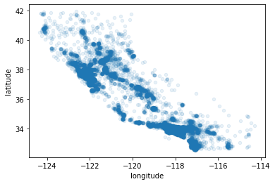
→ Bay area, LA, San Diego, Central Valley 쪽의 집값이 높다.
좀 더 두드러진 패턴 만들어내기
housing.plot(kind = "scatter", x="longitude", y="latitude", alpha=0.4,
            s = housing["population"]/100, label="population", figsize=(10,7),
            c = "median_house_value", cmap=plt.get_cmap("jet"), colorbar=True,
            )
plt.legend()
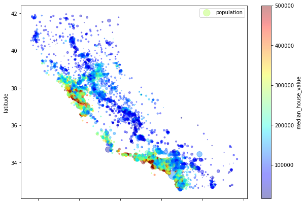
→ 주택 가격이 지역 & 인구밀도와 상관있다는 것을 알 수 있다.
→ 군집 알고리즘을 사용해 주요 군집을 찾고, 군집의 중심까지의 거리를
재는 특성을 추가할 수 있다.
상관관계 조사
코드와 결과
- corr() 함수를 이용한다.
corr_mat = housing.corr()
corr_mat["median_house_value"].sort_values(ascending=False)

"""
결과
median_house_value    1.000000
median_income         0.687160
total_rooms           0.135097
housing_median_age    0.114110
households            0.064506
total_bedrooms        0.047689
population           -0.026920
longitude            -0.047432
latitude             -0.142724
Name: median_house_value, dtype: float64

"""
- 상관계수의 시각화
from pandas.plotting import scatter_matrix

attributes = ["median_house_value", "median_income",
             "total_rooms", "housing_median_age"]

scatter_matrix(housing[attributes], figsize=(12,8))
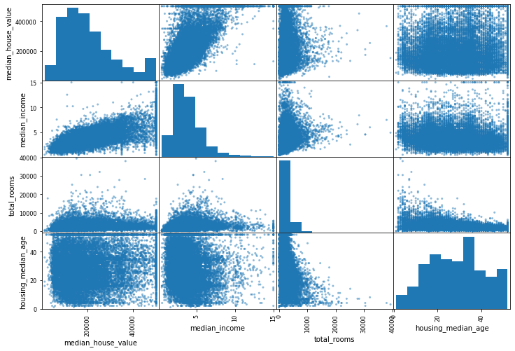
이 중에서 “중간 주택 가격”과 “중간 소득” 간의 상관관계를 보자.
housing.plot(kind = "scatter", x = "median_income",
            y = "median_house_value", alpha = 0.1)
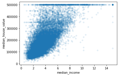
- 결과 해석
- 상관관계가 너무 강하다
- 일부 값들이 수평선으로 잘 보인다. (이상한 데이터)
- 데이터의 모양이 위처럼 이상하다면 재조정을 해야 한다.
특성 조합으로 실험
-
여러가지 데이터들의 특성 조합을 실험해 보기
ex. 가구 당 방 갯수
코드와 결과
pythonhousing["rooms_per_household"] = housing["total_rooms"] / housing["households"] housing["bedrooms_per_room"] = housing["total_bedrooms"] / housing["total_rooms"] housing["population_per_household"] = housing["population"] / housing["households"] corr_matrix = housing.corr() corr_matrix["median_house_value"].sort_values(ascending=False)# 결과 median_house_value 1.000000 median_income 0.687160 rooms_per_household 0.146285 total_rooms 0.135097 housing_median_age 0.114110 households 0.064506 total_bedrooms 0.047689 population_per_household -0.021985 population -0.026920 longitude -0.047432 latitude -0.142724 bedrooms_per_room -0.259984 Name: median_house_value, dtype: float64
5. 머신러닝 알고리즘을 위한 데이터 준비
- 먼저 원래 훈련 세트로 복원.
- 예측 변수와 타깃값에 같은 변형을 적용하지 않기 위해 예측 변수와 레이블을 분리.
housing = strat_train_set.drop("median_house_value", axis=1)
housing_labels = strat_train_set["median_house_value"].copy()
데이터 정제 (수치형)
- 대부분의 머신러닝 알고리즘을 누락된 특성을 다루지 못함.
- 따라서 이를 처리할 수 있는 함수가 필요.
- dropna(), drop(), fillna() 를 사용해 만들 수 있음.
housing.dropna(subset=["total_bedrooms"]) # 옵션 1
housing.drop("total_bedrooms", axis=1) # 옵션 2
median = housing["total_bedrooms"].median() # 옵션 3
housing["total_bedrooms"].fillna(median, inplace=True)
- sklearn의 simpleimputer로 누락된 값 보충
- 누락값 = 특성의 중간값으로 대체
from sklearn.impute import SimpleImputer
imputer = SimpleImputer(strategy = "median")
# imputer로 중간값 계산

housing_num = housing.drop("ocean_proximity", axis=1)
# 수치형이 아닌 ocean_proximity 제거

imputer.fit(housing_num)
# 각 수치형의 중간값 계산
imputer.statistics_
housing_num.median().values

X = imputer.transform(housing_num)
housing_tr = pd.DataFrame(X, columns=housing_num.columns,
                         index = housing_num.index)
텍스트와 범주형 특성 다루기
- 여기서는 범주형이 “ocean_proximity” 하나밖에 없음.
housing_cat = housing[["ocean_proximity"]]
housing_cat.head(10)

# 결과
"""
ocean_proximity
17606	<1H OCEAN
18632	<1H OCEAN
14650	NEAR OCEAN
3230	INLAND
3555	<1H OCEAN
19480	INLAND
8879	<1H OCEAN
13685	INLAND
4937	<1H OCEAN
4861	<1H OCEA
"""
범주형(텍스트) → 숫자로 변환하기
- sklearn의 ordinalEncoder 클래스 이용
from sklearn.preprocessing import OrdinalEncoder
ordinal_encoder = OrdinalEncoder()
housing_cat_encoded = ordinal_encoder.fit_transform(housing_cat)
housing_cat_encoded[:10]

# 카테고리 목록 얻기
ordinal_encoder.categories_
- ocean_proximity의 특성
- 1H OCEAN : 0
- near ocean: 1
- inland : 4
- 0번 지역과 1번 지역의 거리보다 0번 지역과 4번 지역의 거리가 가깝다.
- 따라서, 카테고리별 이진 특성을 만든다.
1H OCEAN 이면 한 특성이 1, 그 외 0
inland 이면 한 특성이 0, 그 외 1 - 이를 one-hot encoding이라고 하며, 새로운 특성을 더미특성이라고 함.
from sklearn.preprocessing import OneHotEncoder
cat_encoder = OneHotEncoder()
housing_cat_1hot = cat_encoder.fit_transform(housing_cat)
housing_cat_1hot

"""
결과: 사이파이 희소행렬(0으로 대부분 채워진 행렬)
<16512x5 sparse matrix of type '<class 'numpy.float64'>'
	with 16512 stored elements in Compressed Sparse Row format>
"""

# 사이파이 희소행렬을 넘파이 배열로
housing_cat_1hot.toarray()

# 카테고리 리스트 추출
cat_encoder.categories_
나만의 변환기
특별한 정제작업을 위해 나만의 변환기를 만들 필요가 있음.
# 나만의 변환기
from sklearn.base import BaseEstimator, TransformerMixin

rooms_ix, bedrooms_ix, population_ix, households_ix = 3, 4, 5, 6
class CombinedAttributesAdder(BaseEstimator, TransformerMixin):
    def __init__(self, add_bedrooms_per_room = True):
        self.add_bedrooms_per_room = add_bedrooms_per_room
    def fit(self, X, y=None):
        return self
    def transform(self, X):
        rooms_per_household = X[:, rooms_ix] / X[:, households_ix]
        population_per_household = X[:, population_ix] / X[:, households_ix]
        if self.add_bedrooms_per_room:
            bedrooms_per_room = X[:, bedrooms_ix] / X[:, rooms_ix]
            return np.c_[X, rooms_per_household, population_per_household,
                        bedrooms_per_room]

        else:
            return np.c_[X, rooms_per_household, population_per_household]

attr_adder = CombinedAttributesAdder(add_bedrooms_per_room = False)
housing_extra_attribs = attr_adder.transform(housing.values)
특성 스케일링
머신러닝 알고리즘은 입력 숫자 특성들의 스케일이 많이 다르면 잘 작동하지 않음.
따라서 특성의 범위를 잘 조정해야 함.
- min-max 스케일링 = 정규화
- 0~1 사이에 들어오도록 값 조정
- 표준화
- 평균을 빼고 분산이 1이 되도록 조정
변환 파이프라인
변환 단계가 많을 때는 연속된 변환을 순서대로 처리해야 한다.
# 변환 파이프라인
from sklearn.pipeline import Pipeline
from sklearn.preprocessing import StandardScaler

num_pipeline = Pipeline([
        ('imputer', SimpleImputer(strategy="median")),
        ('attribs_adder', CombinedAttributesAdder()),
        ('std_scaler', StandardScaler()),
    ])

# 파이프라인은 이름과 추정기를 쌍으로 받는다.
# 마지막 단계에서만 변환기와 추정기를 모두 사용 가능.
# 그 전까지는 변환기만 사용 가능.

housing_num_tr = num_pipeline.fit_transform(housing_num)
housing_num_tr

"""
결과
array([[-0.94135046,  1.34743822,  0.02756357, ...,  0.01739526,
         0.00622264, -0.12112176],
       [ 1.17178212, -1.19243966, -1.72201763, ...,  0.56925554,
        -0.04081077, -0.81086696],
       [ 0.26758118, -0.1259716 ,  1.22045984, ..., -0.01802432,
        -0.07537122, -0.33827252],
       ...,
       [-1.5707942 ,  1.31001828,  1.53856552, ..., -0.5092404 ,
        -0.03743619,  0.32286937],
       [-1.56080303,  1.2492109 , -1.1653327 , ...,  0.32814891,
        -0.05915604, -0.45702273],
       [-1.28105026,  2.02567448, -0.13148926, ...,  0.01407228,
         0.00657083, -0.12169672]])
"""
사이킷런에서는 Pipeline 클래스를 사용한다.
- 하나의 변환기로 범주형/수치형 모두 처리하는 ColumnTransformer 사용.
from sklearn.compose import ColumnTransformer

num_attribs = list(housing_num) # 수치형 리스트
cat_attribs = ["ocean_proximity"] # 범주형 리스트

full_pipeline = ColumnTransformer([
        ("num", num_pipeline, num_attribs),
        ("cat", OneHotEncoder(), cat_attribs),
    ])
"""
수치형은 아까 만든 파이프라인에 넣어준다. (밀집행렬 반환)
범주형은 OneHotEncoder()에 넣어준다. (희소행렬 반환)

full_pipeline은 밀집/희소 행렬이 섞이면 최종 행렬의
밀집 정도를 추정한다. 임계값보다 낮으면 희소행렬, 그렇지 않으면
밀집 행렬을 반환한다.
"""
housing_prepared = full_pipeline.fit_transform(housing)
housing_prepared
6. 모델 선택과 훈련
훈련 세트에서 훈련
선형회귀 모델 훈련
from sklearn.linear_model import LinearRegression

lin_reg = LinearRegression()
lin_reg.fit(housing_prepared, housing_labels)
- 어느 정도의 정확성을 보장하는 예측이 나왔다.
some_data = housing.iloc[:5]
some_labels = housing_labels.iloc[:5]
some_data_prepared = full_pipeline.transform(some_data)
print("예측:", lin_reg.predict(some_data_prepared))
print("레이블:", list(some_labels))
- 과연 이 모델은 어느 정도의 오차를 가지고 있는가? RMSE 측정
# MSE 측정
from sklearn.metrics import mean_squared_error as mse
housing_predictions = lin_reg.predict(housing_prepared)
lin_mse = mse(housing_labels, housing_predictions)
lin_rmse = np.sqrt(lin_mse)
print(lin_rmse)

# 결과: 68628.19819848922
- 예측 오차가 약 $68628 → 과소적합된 사례
결정트리 모델 훈련
from sklearn.tree import DecisionTreeRegressor
tree_reg = DecisionTreeRegressor()
tree_reg.fit(housing_prepared, housing_labels)

housing_predictions = tree_reg.predict(housing_prepared)
tree_mse = mse(housing_labels, housing_predictions)
tree_rmse = np.sqrt(tree_mse)
print(tree_rmse)

# 결과 : 0.0
- 예측 오차가 0 ⇒ 과대적합된 사례 (이런 모델은 없는거나 마찬가지!)
교차검증
- 두 모델 중 어느 것이 적합한지 판단하기
- k-fold cross-validation : 10개의 fold로 훈련 세트를 분할. 이후 결정 트리모델을 10번 훈련 & 평가.
결정트리 교차검증
from sklearn.model_selection import cross_val_score
scores = cross_val_score(tree_reg, housing_prepared, housing_labels,
                        scoring = "neg_mean_squared_error", cv=10)
tree_rmse_scores = np.sqrt(-scores)

def display_scores(scores):
    print("점수", scores)
    print("평균:", scores.mean())
    print("표준편차:", scores.std())

display_scores(tree_rmse_scores)
결과를 보면 다음과 같다.
"""
결과 : 별로 좋지 않다.
점수
[69327.01708558 65486.39211857 71358.25563341 69091.37509104
 70570.20267046 75529.94622521 69895.20650652 70660.14247357
 75843.74719231 68905.17669382]
평균: 70666.74616904806
표준편차: 2928.322738055112
"""
선형회귀 교차검증
lin_scores = cross_val_score(lin_reg, housing_prepared, housing_labels,
                            scoring = "neg_mean_squared_error", cv=10)
lin_rmse_scores = np.sqrt(-lin_scores)
display_scores(lin_rmse_scores)
결과는 다음과 같다.
"""
결과 : 조금 더 낫다
점수 :
[66782.73843989 66960.118071   70347.95244419 74739.57052552
 68031.13388938 71193.84183426 64969.63056405 68281.61137997
 71552.91566558 67665.10082067]
평균: 69052.46136345083
표준편차: 2731.6740017983443
"""
결정트리 모델이 더 과대적합되었다고 볼 수 있다.
랜덤포레스트 모델의 교차검증
from sklearn.ensemble import RandomForestRegressor

forest_reg = RandomForestRegressor(n_estimators=100, random_state=42)
forest_reg.fit(housing_prepared, housing_labels)

housing_predictions = forest_reg.predict(housing_prepared)
forest_mse = mean_squared_error(housing_labels, housing_predictions)
forest_rmse = np.sqrt(forest_mse)
forest_rmse

from sklearn.model_selection import cross_val_score

forest_scores = cross_val_score(forest_reg, housing_prepared, housing_labels,
                                scoring="neg_mean_squared_error", cv=10)
forest_rmse_scores = np.sqrt(-forest_scores)
display_scores(forest_rmse_scores)

scores = cross_val_score(lin_reg, housing_prepared, housing_labels, scoring="neg_mean_squared_error", cv=10)
pd.Series(np.sqrt(-scores)).describe()
7. 모델 세부 튜닝
그리드 탐색
하이퍼파라미터 자동 조정하는 것.
from sklearn.model_selection import GridSearchCV

param_grid = [
    # 12(=3×4)개의 하이퍼파라미터 조합을 시도.
    {'n_estimators': [3, 10, 30], 'max_features': [2, 4, 6, 8]},
    # bootstrap은 False로 하고 6(=2×3)개의 조합을 시도합니다.
    {'bootstrap': [False], 'n_estimators': [3, 10], 'max_features': [2, 3, 4]},
  ]

forest_reg = RandomForestRegressor(random_state=42)
# 다섯 개의 폴드로 훈련하면 총 (12+6)*5=90번의 훈련 실현.
grid_search = GridSearchCV(forest_reg, param_grid, cv=5,
                           scoring='neg_mean_squared_error',
                           return_train_score=True)
grid_search.fit(housing_prepared, housing_labels)

grid_search.best_params_
grid_search.best_estimator_

# 평가 점수 확인
cvres = grid_search.cv_results_
for mean_score, params in zip(cvres["mean_test_score"], cvres["params"]):
    print(np.sqrt(-mean_score), params)
pd.DataFrame(grid_search.cv_results_)
랜덤 탐색
하이퍼파라미터 탐색 공간이 커질 때 사용하는 기법
앙상블 탐색
모델을 세밀하게 튜닝하는 또 다른 방법은 최상의 모델을 연결해보는 것.
모델의 그룹이 최상의 단일 모델보다 더 나은 성능 발휘할 때가 많음.
자세한 내용은 7장에서 → 클릭!
최상의 모델과 오차 분석
- 최상의 모델을 분석해 모델 통찰.
- 여기서는 RandomForestRegressor를 통해 각 특성의 상대적 중요도를 이야기해줌
feature_importances = grid_search.best_estimator_.feature_importances_
feature_importances
array([6.96542523e-02, 6.04213840e-02, 4.21882202e-02, 1.52450557e-02,
       1.55545295e-02, 1.58491147e-02, 1.49346552e-02, 3.79009225e-01,
       5.47789150e-02, 1.07031322e-01, 4.82031213e-02, 6.79266007e-03,
       1.65706303e-01, 7.83480660e-05, 1.52473276e-03, 3.02816106e-03])
- (중요도, 특성이름) 순으로 표시
extra_attribs = ["rooms_per_hhold", "pop_per_hhold", "bedrooms_per_room"]
cat_encoder = full_pipeline.named_transformers_["cat"]
cat_one_hot_attribs = list(cat_encoder.categories_[0])
attributes = num_attribs + extra_attribs + cat_one_hot_attribs
sorted(zip(feature_importances, attributes), reverse=True)
"""
결과
[(0.36615898061813423, 'median_income'),
 (0.16478099356159054, 'INLAND'),
 (0.10879295677551575, 'pop_per_hhold'),
 (0.07334423551601243, 'longitude'),
 (0.06290907048262032, 'latitude'),
 (0.056419179181954014, 'rooms_per_hhold'),
 (0.053351077347675815, 'bedrooms_per_room'),
 (0.04114379847872964, 'housing_median_age'),
 (0.014874280890402769, 'population'),
 (0.014672685420543239, 'total_rooms'),
 (0.014257599323407808, 'households'),
 (0.014106483453584104, 'total_bedrooms'),
 (0.010311488326303788, '<1H OCEAN'),
 (0.0028564746373201584, 'NEAR OCEAN'),
 (0.0019604155994780706, 'NEAR BAY'),
 (6.0280386727366e-05, 'ISLAND')]
"""
이걸 바탕으로 덜 중요한 특성들을 제외할 수 있음.
테스트 세트로 시스템 평가하기
- full_pipeline을 사용해 데이터 변환
- 이후 최종 모델 평가
final_model = grid_search.best_estimator_

X_test = strat_test_set.drop("median_house_value", axis=1)
y_test = strat_test_set["median_house_value"].copy()

X_test_prepared = full_pipeline.transform(X_test)
final_predictions = final_model.predict(X_test_prepared)

final_rmse = np.sqrt(mse(y_test, final_predictions))
final_rmse
신뢰 구간 계산
from scipy import stats
confidence = 0.95
squared_errors = (final_predictions - y_test) ** 2
np.sqrt(stats.t.interval(confidence, len(squared_errors) - 1,
                         loc=squared_errors.mean(),
                         scale=stats.sem(squared_errors)))
"""
결과값: array([45893.36082829, 49774.46796717])
"""
8. 론칭, 모니터링, 시스템 유지 보수
- 론칭: 웹앱에 넣으면 된다. (플라스크, 스프링 등등)
- 구글 클라우드에 뿌리든, AWS를 이용하든 배포는 자유.
- 다만, 그 이후 모니터링도 필수다.